Surface Plots for Two-Way Interactions

Makes surface plots to display interactions between two continuous variables

DAintfun(
  obj,
  varnames,
  theta = 45,
  phi = 10,
  xlab = NULL,
  ylab = NULL,
  zlab = NULL,
  hcols = NULL,
  ...
)

Arguments

obj	A model object of class lm
varnames	A two-element character vector where each element is the name of a variable involved in a two-way interaction.
theta	Angle defining the azimuthal viewing direction to be passed to persp
phi	Angle defining the colatitude viewing direction to be passed to persp
xlab	Optional label to put on the x-axis, otherwise if NULL, it will take the first element of varnames
ylab	Optional label to put on the y-axis, otherwise if NULL, it will take the second element of varnames
zlab	Optional label to put on the z-axis, otherwise if NULL, it will be ‘Predictions’
hcols	Vector of four colors to color increasingly high density areas
...	Other arguments to be passed down to the initial call to persp

Value

x1

Values of the first element of varnames used to make predictions.

x2

Values of the second element of varnames used to make predictions.

pred

The predictions based on the values x1 and x2.

graph

A graph is produced, but no other information is returned.

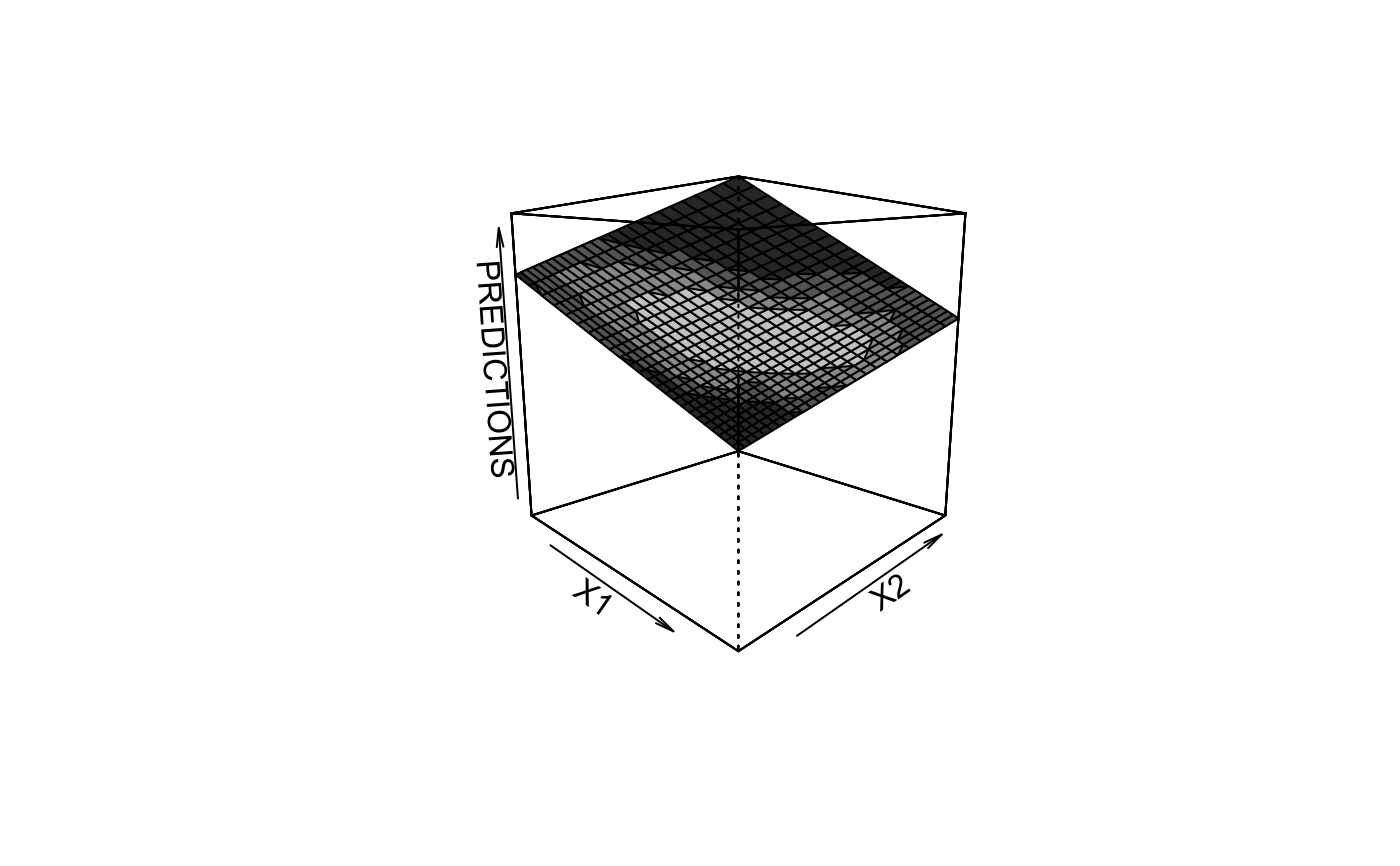
Details

This function makes a surface plot of an interaction between two continuous covariates. If the model is
$$y_{i} = b_{0} + b_{1}x_{i1} + b_{2}x_{i2} + b_{3}x_{i1}\times x_{i2} + \ldots + e_{i},$$
this function plots \(b_{1}x_{i1} + b_{2}x_{i2} + b_{3}x_{i1}\times x_{i2}\) for values over the range of \(X_{1}\) and \(X_{2}\). The highest 75%, 50% and 25% of the bivariate density of \(X_{1}\) and \(X_{2}\) (as calculated by sm.density from the sm package) are colored in with colors of increasing gray-scale.

Examples

data(InteractionEx)
mod <- lm(y ~ x1*x2 + z, data=InteractionEx)
DAintfun(mod, c("x1", "x2"))