Conditional Effects Plots for Interactions in Linear Models

Generates two conditional effects plots for two interacted continuous covariates in linear models.

DAintfun2(
  obj,
  varnames,
  varcov = NULL,
  rug = TRUE,
  ticksize = -0.03,
  hist = FALSE,
  hist.col = "gray75",
  nclass = c(10, 10),
  scale.hist = 0.5,
  border = NA,
  name.stem = "cond_eff",
  xlab = NULL,
  ylab = NULL,
  plot.type = "screen"
)

Arguments

obj	A model object of class lm
varnames	A two-element character vector where each element is the name of a variable involved in a two-way interaction.
varcov	A variance-covariance matrix with which to calculate the conditional standard errors. If NULL, it is calculated with vcov(obj).
rug	Logical indicating whether a rug plot should be included.
ticksize	A scalar indicating the size of ticks in the rug plot (if included) positive values put the rug inside the plotting region and negative values put it outside the plotting region.
hist	Logical indicating whether a histogram of the x-variable should be included in the plotting region.
hist.col	Argument to be passed to polygon indicating the color of the histogram bins.
nclass	vector of two integers indicating the number of bins in the two histograms, which will be passed to hist.
scale.hist	A scalar in the range (0,1] indicating how much vertical space in the plotting region the histogram should take up.
border	Argument passed to polygon indicating how the border of the histogram bins should be printed (NA for no border).
name.stem	A character string giving filename to which the appropriate extension will be appended
xlab	Optional vector of length two giving the x-labels for the two plots that are generated. The first element of the vector corresponds to the figure plotting the conditional effect of the first variable in varnames given the second and the second element of the vector corresponds to the figure plotting the conditional effect of the second variable in varnames conditional on the first.
ylab	Optional vector of length two giving the y-labels for the two plots that are generated. The first element of the vector corresponds to the figure plotting the conditional effect of the first variable in varnames given the second and the second element of the vector corresponds to the figure plotting the conditional effect of the second variable in varnames conditional on the first.
plot.type	One of ‘pdf’, ‘png’, ‘eps’ or ‘screen’, where the one of the first three will produce two graphs starting with name.stem written to the appropriate file type and the third will produce graphical output on the screen.

Value

graphs

Either a single graph is printed on the screen (using par(mfrow=c(1,2))) or two figures starting with name.stem are produced where each gives the conditional effect of one variable based on the values of another.

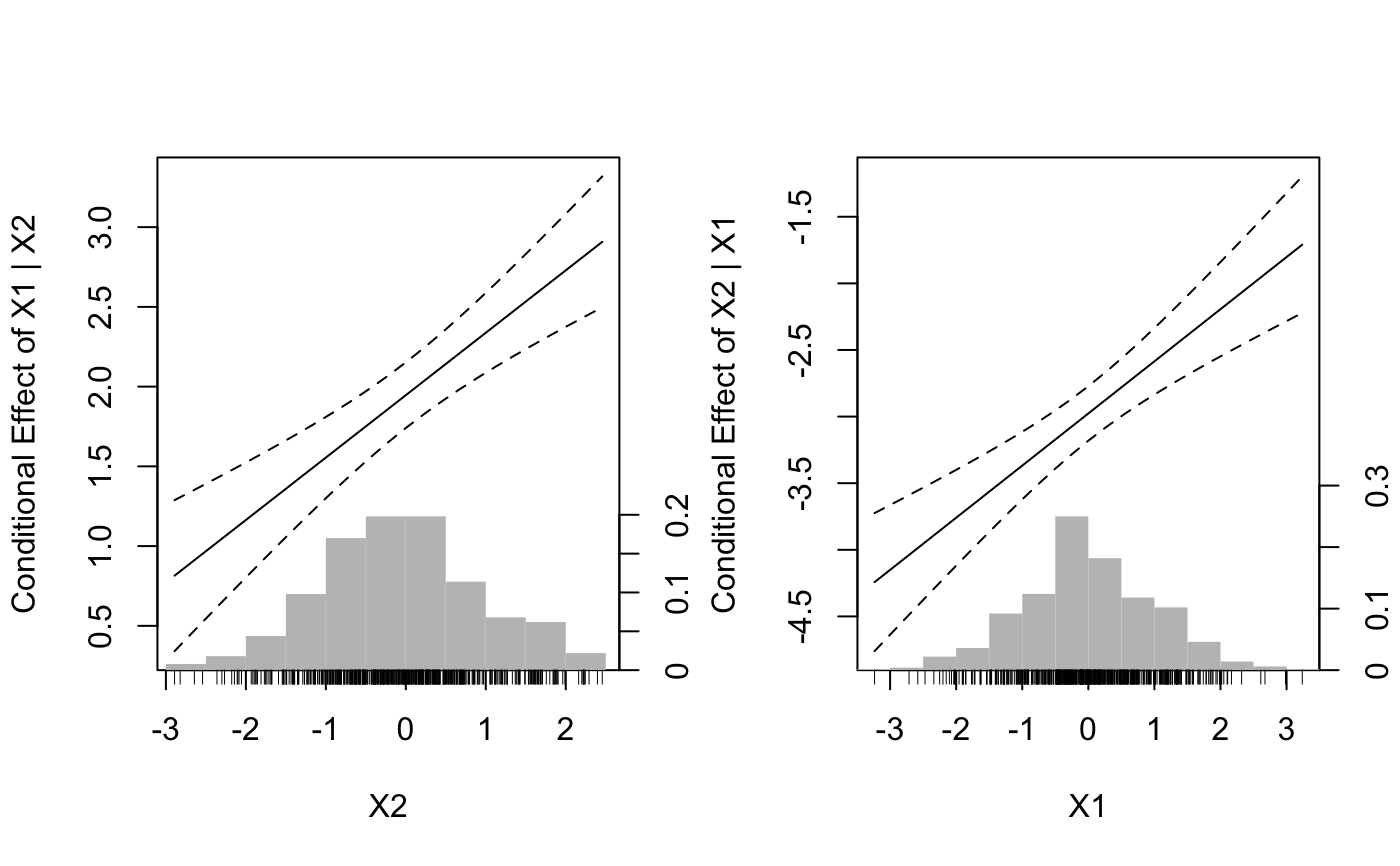
Details

This function produces graphs along the lines suggested by Brambor, Clark and Golder (2006) and Berry, Golder and Milton (2012), that show the conditional effect of one variable in an interaction given the values of the conditioning variable. This is an alternative to the methods proposed by John Fox in his effects package, upon which this function depends heavily.

Specifically, if the model is
$$y_{i} = b_{0} + b_{1}x_{i1} + b_{2}x_{i2} + b_{3}x_{i1}\times x_{i2} + \ldots + e_{i},$$
this function plots calculates the conditional effect of \(X_{1}\) given \(X_{2}\)
$$\frac{\partial y}{\partial X_{1}} = b_{1} + b_{3}X_{2}$$ and the variances of the conditional effects
$$V(b_{1} + b_{3}X_{2}) = V(b_{1} + X_{2}^{2}V(b_{3}) + 2(1)(X_{2})V(b_{1},b_{3}))$$ for different values of \(X_{2}\) and then switches the places of \(X_{1}\) and \(X_{2}\), calculating the conditional effect of \(X_{2}\) given a range of values of \(X_{1}\). 95% confidence bounds are then calculated and plotted for each conditional effects along with a horizontal reference line at 0.

References

Brambor, T., W.R. Clark and M. Golder. (2006) Understanding Interaction Models: Improving Empirical Analyses. Political Analysis 14, 63-82.
Berry, W., M. Golder and D. Milton. (2012) Improving Tests of Theories Positing Interactions. Journal of Politics.

Examples

data(InteractionEx)
mod <- lm(y ~ x1*x2 + z, data=InteractionEx)
DAintfun2(mod, c("x1", "x2"), hist=TRUE, scale.hist=.3)